05 — Turning (Figure 5)¶

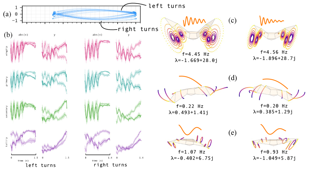
This notebook reproduces Figure 5: DMD analysis of left and right turns during obstacle avoidance flights. The turning data comprises flights by one individual, Toothless, split by turn direction.

We show that DMD captures mirrored banking modes as well as an asymmetric turning mode that distinguishes left from right manoeuvres.

In [1]:

%load_ext autoreload
%autoreload 2
%matplotlib widget
%config InlineBackend.figure_format='svg'

import matplotlib.pyplot as plt
import numpy as np
from morphing_birds import (
    Hawk3D,
    animate,
    animate_compare,
    animate_plotly_compare,
    plot_plotly_with_trace,
)

from birddmd import compute_rmse, plot_mode_dynamics, reconstruct, run_dmd

%load_ext autoreload %autoreload 2 %matplotlib widget %config InlineBackend.figure_format='svg' import matplotlib.pyplot as plt import numpy as np from morphing_birds import ( Hawk3D, animate, animate_compare, animate_plotly_compare, plot_plotly_with_trace, ) from birddmd import compute_rmse, plot_mode_dynamics, reconstruct, run_dmd

In [2]:

hawk3d = Hawk3D("../data/mean_hawk_shape.csv")
average_shape = hawk3d.markers
n_markers = 8
N_MODES = 6

D = 2

hawk3d = Hawk3D("../data/mean_hawk_shape.csv") average_shape = hawk3d.markers n_markers = 8 N_MODES = 6 D = 2

1 — Load turning data¶

We load left and right turn data for Toothless at 9 m. Both conditions come from a single combined full-flight file (Full_9mObstacleToothless_BilateralNoRot.npz), split by the Turn column and time-filtered to match the original analysis.

The preparation script (scripts/prepare_turning.py) splits the combined file by turn direction and applies condition-specific time filters. Expand the cell below to review the pipeline.

In [3]:

# %load scripts/prepare_turning.py

# %load scripts/prepare_turning.py

In [4]:

loaded_dataset = np.load("../data/processed/Toothless_turning_binned.npz")
conditions = {
    "Left turn": ("markers_left", "times_left"),
    "Right turn": ("markers_right", "times_right"),
}

all_results = {}

for label, (ii_markers, ii_times) in conditions.items():
    print(f"\n--- {label} ---")
    markers = loaded_dataset[ii_markers]
    times = loaded_dataset[ii_times]

    result = run_dmd(
        data=markers,
        times=times,
        n_modes=N_MODES,
        d=D,
        eig_constraints={"conjugate_pairs"},
        n_markers=n_markers,
        average_shape=average_shape,
        verbose=False,
    )

    all_results[label] = {
        "result": result,
        "markers": markers,
        "times": times,
    }

    print(f"  {markers.shape[0]} frames, {result.n_pairs} pairs")
    for idx in range(result.n_pairs):
        print(f"  Pair {idx + 1}: {result.pair_frequency(idx):.2f} Hz")

loaded_dataset = np.load("../data/processed/Toothless_turning_binned.npz") conditions = { "Left turn": ("markers_left", "times_left"), "Right turn": ("markers_right", "times_right"), } all_results = {} for label, (ii_markers, ii_times) in conditions.items(): print(f"\n--- {label} ---") markers = loaded_dataset[ii_markers] times = loaded_dataset[ii_times] result = run_dmd( data=markers, times=times, n_modes=N_MODES, d=D, eig_constraints={"conjugate_pairs"}, n_markers=n_markers, average_shape=average_shape, verbose=False, ) all_results[label] = { "result": result, "markers": markers, "times": times, } print(f" {markers.shape[0]} frames, {result.n_pairs} pairs") for idx in range(result.n_pairs): print(f" Pair {idx + 1}: {result.pair_frequency(idx):.2f} Hz")

--- Left turn ---
  270 frames, 3 pairs
  Pair 1: 4.56 Hz
  Pair 2: 0.93 Hz
  Pair 3: 0.20 Hz

--- Right turn ---
  260 frames, 3 pairs
  Pair 1: 4.45 Hz
  Pair 2: 1.07 Hz
  Pair 3: 0.22 Hz

2 — Mode dynamics comparison¶

The dynamics plots below show the temporal evolution of each conjugate pair for each condition. Look for modes whose amplitude or phase differs between left and right turns — these capture the asymmetric banking component of the manoeuvre.

In [5]:

for label, res in all_results.items():
    print(f"\n{label}")
    fig = plot_mode_dynamics(
        res["result"].times[1:],
        res["result"],
        title_prefix=label,
        y_lim=None,
        axes_visible=True,
    )
    clean = label.lower().replace(" ", "_").replace("(", "").replace(")", "")
    fig.savefig(
        f"figures/05_dynamics_{clean}.svg",
        format="svg",
    )

for label, res in all_results.items(): print(f"\n{label}") fig = plot_mode_dynamics( res["result"].times[1:], res["result"], title_prefix=label, y_lim=None, axes_visible=True, ) clean = label.lower().replace(" ", "_").replace("(", "").replace(")", "") fig.savefig( f"figures/05_dynamics_{clean}.svg", format="svg", )

Left turn
Pair 1 (0,1) Frequency: 4.56 Hz | f=4.56 Hz | λ=-1.860+28.671j
Pair 2 (2,3) Frequency: 0.93 Hz | f=0.93 Hz | λ=-1.049+5.868j
Pair 3 (4,5) Frequency: 0.20 Hz | f=0.20 Hz | λ=0.385+1.286j

Figure

Right turn
Pair 1 (0,1) Frequency: 4.45 Hz | f=4.45 Hz | λ=-1.669+27.953j
Pair 2 (2,3) Frequency: 1.07 Hz | f=1.07 Hz | λ=-0.402+6.746j
Pair 3 (4,5) Frequency: -0.22 Hz | f=-0.22 Hz | λ=0.493-1.411j

Figure

3 — Visualise turning modes¶

We first compare the wingbeat mode (pair 0) for left and right turns side by side — the two reconstructions should appear as approximate mirror images, reflecting the bilateral symmetry of the banking motion.

We then decompose the right turn into individual mode contributions, following the same approach as notebook 01.

In [6]:

# Compare left and right turn first mode pair (wingbeat)
# hawk3d = Hawk3D("../data/mean_hawk_shape.csv")

left_res = all_results["Left turn"]["result"]
right_res = all_results["Right turn"]["result"]

# Reconstruct wingbeat mode for each
left_wb = reconstruct(left_res, pairs=[0])
right_wb = reconstruct(right_res, pairs=[0])

# Trim to equal length
min_len = min(left_wb.shape[0], right_wb.shape[0])
left_wb = left_wb[:min_len]
right_wb = right_wb[:min_len]

# animate_plotly_compare(
#     hawk3d,
#     keypoints_frames_list=[left_wb, right_wb],
#     colours=["blue", "red"],
# )

# Compare left and right turn first mode pair (wingbeat) # hawk3d = Hawk3D("../data/mean_hawk_shape.csv") left_res = all_results["Left turn"]["result"] right_res = all_results["Right turn"]["result"] # Reconstruct wingbeat mode for each left_wb = reconstruct(left_res, pairs=[0]) right_wb = reconstruct(right_res, pairs=[0]) # Trim to equal length min_len = min(left_wb.shape[0], right_wb.shape[0]) left_wb = left_wb[:min_len] right_wb = right_wb[:min_len] # animate_plotly_compare( # hawk3d, # keypoints_frames_list=[left_wb, right_wb], # colours=["blue", "red"], # )

In [7]:

# # Save left vs right wingbeat comparison as GIF
# hawk3d = Hawk3D("../data/mean_hawk_shape.csv")
# ani = animate_compare(
#     hawk3d, [left_wb, right_wb],
#     colour=["blue", "red"], az=50, el=30,
# )
# ani.save("figures/05_left_vs_right_wingbeat.gif", writer='Pillow', fps=40, dpi=300)
# print("Saved figures/05_left_vs_right_wingbeat.gif")

# # Save left vs right wingbeat comparison as GIF # hawk3d = Hawk3D("../data/mean_hawk_shape.csv") # ani = animate_compare( # hawk3d, [left_wb, right_wb], # colour=["blue", "red"], az=50, el=30, # ) # ani.save("figures/05_left_vs_right_wingbeat.gif", writer='Pillow', fps=40, dpi=300) # print("Saved figures/05_left_vs_right_wingbeat.gif")

In [8]:

# RMSE for each condition
for label, res in all_results.items():
    result = res["result"]
    markers_compare = res["markers"][:-1]
    rmse = compute_rmse(result.reconstruction, markers_compare)
    print(f"{label}: mean RMSE = {np.mean(rmse):.6f} m")

# RMSE for each condition for label, res in all_results.items(): result = res["result"] markers_compare = res["markers"][:-1] rmse = compute_rmse(result.reconstruction, markers_compare) print(f"{label}: mean RMSE = {np.mean(rmse):.6f} m")

Left turn: mean RMSE = 0.029274 m
Right turn: mean RMSE = 0.030195 m

In [9]:

# Reconstruct each conjugate pair separately for the right turn
conjugate_pairs = right_res.conjugate_pairs
n_pairs = len(conjugate_pairs)

pair_colours = ["#DF5D99", "#57B7B0", "#EE7447", "#6B5B95", "#88B04B"][:n_pairs]

mode_keypoints = []
pair_labels = []
for pair_idx in range(n_pairs):
    kp = reconstruct(right_res, pairs=[pair_idx])
    mode_keypoints.append(kp)
    freq = right_res.pair_frequency(pair_idx)
    label = f"{freq:.2f} Hz"
    pair_labels.append(label)
    i, j = conjugate_pairs[pair_idx]
    print(f"  Pair {pair_idx + 1} ({label}): modes ({i},{j})")

# Reconstruct each conjugate pair separately for the right turn conjugate_pairs = right_res.conjugate_pairs n_pairs = len(conjugate_pairs) pair_colours = ["#DF5D99", "#57B7B0", "#EE7447", "#6B5B95", "#88B04B"][:n_pairs] mode_keypoints = [] pair_labels = [] for pair_idx in range(n_pairs): kp = reconstruct(right_res, pairs=[pair_idx]) mode_keypoints.append(kp) freq = right_res.pair_frequency(pair_idx) label = f"{freq:.2f} Hz" pair_labels.append(label) i, j = conjugate_pairs[pair_idx] print(f" Pair {pair_idx + 1} ({label}): modes ({i},{j})")

  Pair 1 (4.45 Hz): modes (0,1)
  Pair 2 (1.07 Hz): modes (2,3)
  Pair 3 (0.22 Hz): modes (4,5)

In [10]:

# Save each right-turn mode pair as a GIF
# hawk3d = Hawk3D("../data/mean_hawk_shape.csv")
# for pair_idx, (kp, label, colour) in enumerate(
#     zip(mode_keypoints, pair_labels, pair_colours)
# ):
#     ani = animate(hawk3d, kp, colour=colour, az=90, el=10)
#     ani.save(
#         f"figures/05_right_turn_mode_{pair_idx}.gif",
#         writer="Pillow", fps=40, dpi=300,
#     )
#     print(f"Saved figures/05_right_turn_mode_{pair_idx}.gif ({label})")

# Save each right-turn mode pair as a GIF # hawk3d = Hawk3D("../data/mean_hawk_shape.csv") # for pair_idx, (kp, label, colour) in enumerate( # zip(mode_keypoints, pair_labels, pair_colours) # ): # ani = animate(hawk3d, kp, colour=colour, az=90, el=10) # ani.save( # f"figures/05_right_turn_mode_{pair_idx}.gif", # writer="Pillow", fps=40, dpi=300, # ) # print(f"Saved figures/05_right_turn_mode_{pair_idx}.gif ({label})")

In [11]:

# Reconstruct each conjugate pair separately for the right turn
conjugate_pairs = left_res.conjugate_pairs
n_pairs = len(conjugate_pairs)

pair_colours = ["#DF5D99", "#57B7B0", "#EE7447", "#6B5B95", "#88B04B"][:n_pairs]

mode_keypoints = []
pair_labels = []
for pair_idx in range(n_pairs):
    kp = reconstruct(left_res, pairs=[pair_idx])
    mode_keypoints.append(kp)
    freq = left_res.pair_frequency(pair_idx)
    label = f"{freq:.2f} Hz"
    pair_labels.append(label)
    i, j = conjugate_pairs[pair_idx]
    print(f"  Pair {pair_idx + 1} ({label}): modes ({i},{j})")

# Reconstruct each conjugate pair separately for the right turn conjugate_pairs = left_res.conjugate_pairs n_pairs = len(conjugate_pairs) pair_colours = ["#DF5D99", "#57B7B0", "#EE7447", "#6B5B95", "#88B04B"][:n_pairs] mode_keypoints = [] pair_labels = [] for pair_idx in range(n_pairs): kp = reconstruct(left_res, pairs=[pair_idx]) mode_keypoints.append(kp) freq = left_res.pair_frequency(pair_idx) label = f"{freq:.2f} Hz" pair_labels.append(label) i, j = conjugate_pairs[pair_idx] print(f" Pair {pair_idx + 1} ({label}): modes ({i},{j})")

  Pair 1 (4.56 Hz): modes (0,1)
  Pair 2 (0.93 Hz): modes (2,3)
  Pair 3 (0.20 Hz): modes (4,5)

In [12]:

# Save each left-turn mode pair as a GIF
# hawk3d = Hawk3D("../data/mean_hawk_shape.csv")
# for pair_idx, (kp, label, colour) in enumerate(
#     zip(mode_keypoints, pair_labels, pair_colours)
# ):
#     ani = animate(hawk3d, kp, colour=colour, az=90, el=10)
#     ani.save(
#         f"figures/05_left_turn_mode_{pair_idx}.gif",
#         writer="Pillow", fps=40, dpi=300,
#     )
#     print(f"Saved figures/05_left_turn_mode_{pair_idx}.gif ({label})")

# Save each left-turn mode pair as a GIF # hawk3d = Hawk3D("../data/mean_hawk_shape.csv") # for pair_idx, (kp, label, colour) in enumerate( # zip(mode_keypoints, pair_labels, pair_colours) # ): # ani = animate(hawk3d, kp, colour=colour, az=90, el=10) # ani.save( # f"figures/05_left_turn_mode_{pair_idx}.gif", # writer="Pillow", fps=40, dpi=300, # ) # print(f"Saved figures/05_left_turn_mode_{pair_idx}.gif ({label})")

In [13]:

# # 3D visualisation of individual modes
# for pair_idx, (kp, label, colour) in enumerate(
#     zip(mode_keypoints, pair_labels, pair_colours)
# ):
#     hawk3d = Hawk3D("../data/mean_hawk_shape.csv")
#     hawk3d.update_keypoints(kp[0])
#
#     fig = plot_plotly_with_trace(hawk3d, keypoints_frames=kp, colour=colour)
#     fig.update_layout(
#         scene=dict(
#             camera=dict(eye=dict(x=0.0, y=1, z=0.3)),
#             xaxis=dict(visible=False, range=[-0.8, 0.8]),
#             yaxis=dict(visible=False, range=[-0.8, 0.8]),
#             zaxis=dict(visible=False, range=[-0.8, 0.8]),
#         ),
#     )
#     fig.show()

# # 3D visualisation of individual modes # for pair_idx, (kp, label, colour) in enumerate( # zip(mode_keypoints, pair_labels, pair_colours) # ): # hawk3d = Hawk3D("../data/mean_hawk_shape.csv") # hawk3d.update_keypoints(kp[0]) # # fig = plot_plotly_with_trace(hawk3d, keypoints_frames=kp, colour=colour) # fig.update_layout( # scene=dict( # camera=dict(eye=dict(x=0.0, y=1, z=0.3)), # xaxis=dict(visible=False, range=[-0.8, 0.8]), # yaxis=dict(visible=False, range=[-0.8, 0.8]), # zaxis=dict(visible=False, range=[-0.8, 0.8]), # ), # ) # fig.show()

In [14]:

# hawk3d = Hawk3D("../data/mean_hawk_shape.csv")

# animate_plotly_compare(
#     hawk3d,
#     keypoints_frames_list=mode_keypoints,
#     colours=pair_colours,
# )

# hawk3d = Hawk3D("../data/mean_hawk_shape.csv") # animate_plotly_compare( # hawk3d, # keypoints_frames_list=mode_keypoints, # colours=pair_colours, # )

Next¶

The next notebook (06_reconstruction_accuracy) validates the three-mode decomposition across 413 individual sequences (not just binned averages), confirming that the mode structure generalises across birds, distances, and conditions.